Machine Learning Notes 4

Gradient descent algorithm for multiple linear regression

(i.e. for linear regression with multiple variables)

Terminology (notation used):

$n$ - this is the number of features (the number of input variables)

$X_1, X_2, \dots, X_n$ - these are the features

$X_j$ - the $j$-th feature ($j = 1,2,\dots,n$)

$Y$ - the target (output) variable

$m$ - the size of the training set (the number of training examples)

$X_j^{(i)}$ - the $i$-th training value from the $j$-th feature ($i = 1,2,\dots,m$)

Let's assume that we have the following features and training examples.

 

#	$X_1$	$X_2$	$X_3$	...	$X_n$	$Y$
1	2100	5	1	...	45	460
2	1400	3	2	...	40	235
3	1530	3	2	...	30	315
...	...	...	...	...	...	...
m	850	2	1	...	35	175

Here we have that $X_1^{(3)} = 1530$, $X_2^{(2)} = 3$, $X_n^{(3)} = 30$, $X_n^{(m)} = 35$

$\overrightarrow{X}^{(i)}$ - this is a row vector of all $i$-th training values (basically the $i$-th row from the table above without the Y values), so this is the $i$-th training example

$\overrightarrow{X}^{(i)} = (X_1^{(i)}, X_2^{(i)}, \dots, X_n^{(i)})$, for $i=1,2,\dots,m$ 

Note: The training examples are the rows from the table above.

The linear regression model for a single feature was defined as follows.

$f_{w,b} = w \cdot x + b \tag{1}$

The linear regression model for multiple features is defined as follows.

$f_{w,b} = \sum_{j=1}^n w_j \cdot x_j + b \tag{2}$

We can rewrite this model in vector notation. Let us denote 

$\overrightarrow {w} = (w_1, w_2, \dots, w_n)$ - this is a row vector of $n$ scalars (these are the weights assigned to the features)

$b$ - this is a scalar (a number), this value $b$ is the bias

$\overrightarrow {x} = (x_1, x_2, \dots, x_n)$ - this is a row vector of $n$ scalars (the input variables to our model)

Then for the multiple linear regression model we obtain

$f_{\overrightarrow{w},b} = \overrightarrow{w} \cdot \overrightarrow{x} + b \tag{3}$

Here $\overrightarrow{w}, \overrightarrow{b}$ are the parameters of the multiple linear regression model.

In this notation $\overrightarrow{w}\cdot \overrightarrow{x}$ is the dot product of the vectors $\overrightarrow{w}$ and $\overrightarrow{x}$ i.e. 

$\overrightarrow{w} \cdot \overrightarrow{x} = \sum_{j=1}^n w_j \cdot x_j \tag{4}$

Note: This is called multiple linear regression, and not multivariate linear regression. The term multivariate linear regression in machine learning is used for something else. 

For example in the table above $Y$ might be the price of a house (in 1000s of US dollars) which we are trying to estimate (i.e. build a model for), $X_1$ might be the size of the house in square feet, $X_2$ might be the number of bedrooms, $X_3$ might be the number of floors, and $X_n$ might be the age of the house in years (let us say n=4). Then one possible linear model for the price (Y) of the house could be as follows: 

$f_{w,b}(x) = 0.1 \cdot x_1 + 4 \cdot x_2 + 10 \cdot x_3 + (-2) \cdot x_4 + 80 \tag{5}$ 

Here we have $b=80$, and this is called the base price. 

We denote 

$\hat{y}^{(j)} = f_{\overrightarrow{w}, b} (x^{(j)}) = \sum_{i=1}^n w_i \cdot x_i^{(j)} + b\tag{6}$ 

This value is the predicted value (by the linear regression model) which 

corresponds to the $j$-th training example (here $j=1,2,\dots,m$). 

We also have 

$y^{(j)}$ - the actual value corresponding to the $j$-th training example ($j=1,2,\dots,m$).

The least mean squares (LMS) cost function is defined as follows 

$$J(\overrightarrow{w},b) = J(w_1, w_2, \dots, w_n, b) = \frac{1}{2m}\sum_{i=1}^m (\hat{y}^{(i)} - y^{(i)})^2 \tag{7}$$

$$J(\overrightarrow{w},b) = \frac{1}{2m}\sum_{i=1}^m (f_{\overrightarrow{w},b}(\overrightarrow{x}^{(i)}) - y^{(i)})^2 \tag{8}$$

$$J(\overrightarrow{w},b) = \frac{1}{2m} \sum_{i=1}^m (w_1 x_1^{(i)} + w_2 x_2^{(i)} + \dots + w_n x_n^{(i)} + b - y ^ {(i)})^2 \tag{9}$$   

So we get that 

$$J(\overrightarrow{w},b) = \frac{1}{2m}\sum_{i=1}^m [  (\sum_{j=1}^n w_j \cdot x_j^{(i)}) + b - y^{(i)}]^2 \tag{10}$$ 

The gradient descent algorithm essentially varies the $w_j$ and $b$ parameters of the model to find the optimal i.e. the minimal value for $J$ (since $J$ is a function of the parameters $b$ and $w_j$, $j=1,2,\dots,n$). 

So we compute 

$$\frac{\partial{J}}{\partial{w_j}} = \frac{1}{m}\sum_{i=1}^m (f_{\overrightarrow{w},b}(\overrightarrow{x}^{(i)}) - y^{(i)}) \cdot x_j^{(i)} \tag{11}$$ 

(here $j=1,2,\dots,n$)

and 

$$\frac{\partial{J}}{\partial{b}} = \frac{1}{m}\sum_{i=1}^m (f_{\overrightarrow{w},b}(\overrightarrow{x}^{(i)}) - y^{(i)}) \tag{12}$$ 

Now that we have formulas for these partial derivatives, the gradient descent algorithm for multiple linear regression goes as follows. 

1. Pick a small positive number $\alpha \gt 0$. 

2. Repeat these four actions until convergence 

2.1. 

$$temporary\_w_{j} = w_{j} - \alpha \cdot \frac{\partial{J}}{\partial{w_j}}$$ for $j=1,2,\dots,n$

(use the partial derivative expression from (11))

2.2.

$$temporary\_b = b - \alpha \cdot \frac{\partial{J}}{\partial{b}}$$

(use the partial derivative expression from (12))

2.3.

$$w_j = temporary\_w_j$$ for $j=1,2,\dots,n$

2.4. 

$$b = temporary\_b$$

• The temporary variables here are used to underline the fact that the algorithm is doing a simultaneous update of the (n+1) parameters $w_1, w_2, \dots, w_n, b$. That means we should not change any of the parameters before we have computed the new values for all the parameters. 

• Convergence means that the values of the (n+1) parameters $w_1, w_2, \dots, w_n, b$ have settled i.e.  it means they all change by very little after certain number of iterations (say after K iterations/steps). To detect convergence we can use some sort of threshold e.g. we can assume the algorithm has converged if all parameters change only by less then 0.05% after certain number of iterations/steps.

This completes our description of the gradient descent algorithm for multiple linear regression.

Generating a minimal set algebra from a given set of sets

This is a Python program which generates the minimal set algebra which contains all the elements/sets of the set C. In this program Omega is the universal set. Then C is a subset of the powerset of Omega. The program generates the minimal set algebra C3 which contains all the elements of C. A set algebra is also known as a field of sets. Of course here Omega and C are both finite sets. 

       
import itertools as it

Empty = frozenset({})


def main():
    # Omega ---> the universal set
    Omega = frozenset({1, 2, 3, 4, 5, 6})

    # C ---> a set of subsets of Omega

    # C = {frozenset({1}), frozenset({1,3})}
    # C = {frozenset({1,2}), frozenset({2,3,4}), frozenset({5})}

    C = {frozenset({1, 2}), frozenset({2, 3, 5})}

    # Now we generate the sets C1, C2, C3

    # C3 is the minimal boolean algebra
    # which contains all the elements of C

    print("=" * 60)
    C1 = gen_C1(Omega, C)
    C2 = gen_C2(Omega, C1)
    C3 = gen_C3(Omega, C2)

    print("The set of sets C is given as input.")
    print("Size: ", len(C), "---> C = ", make_lst(C))
    print("Added all complements to C ---> result: C1")
    print("Size: ", len(C1), "---> C1 = ", make_lst(C1))

    print("Added all intersections to C1 ---> result: C2")
    print("Size: ", len(C2), "---> C2 = ", make_lst(C2))

    print("Added all unions of disjoint sets to C2 ---> result: C3")
    print("Size: ", len(C3), "---> C3 = ", make_lst(C3))

    print("Checking if C3 is indeed a set algebra ---> ", is_set_algebra(Omega, C3))

    print("=" * 60)


def make_lst(C):
    P = []
    for A in C:
        P.append(str(set(A)) if not Empty == A else "{}")
    return P


def powerset(Omega):
    n = len(Omega)
    ps = set({})

    for k in range(0, n + 1):
        z = it.combinations(Omega, k)
        for t in z:
            ps.add(frozenset(t))

    return ps


def gen_C1(Omega, C):
    ps = powerset(Omega)
    C1 = frozenset({})
    C1 = C1 | {Empty}
    C1 = C1 | {Omega}
    for A in C:
        C1 = C1 | {A}
        C1 = C1 | {Omega - A}

    return C1


def gen_C2(Omega, C1):
    P = Empty
    k = 0

    while (True):
        k = k + 1
        sz1 = len(P)
        Z = Empty
        S = C1 if k == 1 else P

        for A in S:
            for B in S:
                Z = Z | {A & B}

        P = P | Z

        sz2 = len(P)
        if sz2 == sz1:
            break

    return P


def gen_C3(Omega, C2):
    P = Empty
    k = 0

    while True:
        k = k + 1
        sz1 = len(P)
        Z = Empty
        S = C2 if k == 1 else P

        for A in S:
            for B in S:
                # print("A=",A)
                # print("B=",B)
                if A & B == Empty or A & B == A or A & B == B:
                    # print("Adding to Z ...")
                    Z = Z | {A | B}

        P = P | Z

        sz2 = len(P)
        if sz2 == sz1:
            break

    return P


def is_set_algebra(Omega, U):
    if Omega not in U:
        return False

    if Empty not in U:
        return False

    for A in U:
        B = Omega - A
        if B not in U:
            return False

    for A in U:
        for B in U:
            if not (A | B in U):
                return False
            if not (A & B in U):
                return False

    return True


if __name__ == "__main__":
    main()


       

Equation of a plane passing through 3 points

Equation of a plane passing through 3 points

Let's assume we're given 3 distinct points in the 3-dimensional space and these points are not collinear. On a side note, this implies the given 3 points are also distinct.

Let's also assume that their coordinates in some 3-dimensional coordinate system $S = \{O,\overrightarrow{e_1},\overrightarrow{e_2},\overrightarrow{e_3}\}$ are as follows.  

$P_1 = (x_1, y_1, z_1)$

$P_2 = (x_2, y_2, z_2)$

$P_3 = (x_3, y_3, z_3)$

The coordinate system $S$ does not need to be orthogonal. 

Then the equation of the plane passing through these points is as follows. 

$$\begin{vmatrix}x-x_1&y-y_1&z-z_1\\x_2-x_1&y_2-y_1&z_2-z_1\\x_3-x_1&y_3-y_1&z_3-z_1\end{vmatrix} = 0$$

Note: This is a determinant in the expression above.

Machine Learning Notes 3

Gradient descent algorithm

for univariate linear regression

(i.e. for linear regression with one variable)

Let $J(w,b)$ be any cost function of two variables. If we want to be specific, we can assume that $J(w,b)$ is the usual mean squared error cost function from the univariate linear regression model.

See here: ML Notes 2

1) The algorithm first sets two arbitrary values into $w$ and $b$ (e.g. $w := 0,\ b := 0$)

2) Then a loop begins. At each step of that loop the algorithm applies these two updates simultaneously 

2.1) $w := w - \alpha \cdot \frac{\partial J}{\partial w}(w,b)$

2.2) $b := b - \alpha \cdot \frac{\partial J}{\partial b}(w,b)$

Here $\alpha$ is some small positive number e.g. $\alpha=0.01$

This number $\alpha$ is called the learning rate. It controls the size of the step which the algorithm takes downhill in each iteration of the loop.

3) The loop repeats step 2) until the values of $(w,b)$ eventually settle at some point $(w_0, b_0)$. Settle means that after a number of steps, the values of $w$ and $b$ no longer change much with each additional step of the algorithm. At that point, the algorithm exits the loop. The point $(w_0, b_0)$ is the point where $J(w,b)$ has a local minimum. We also say that the algorithm converges to the point $(w_0, b_0)$ after a number of steps.

Note 1: A correct implementation ensures that the updates in step 2) are done simultaneously. What does that mean? That means in the two right hand sides of the assignments 2.1) and 2.2), we should make sure we are using "the old values" of $w$ and $b$. Usually this is implemented in the following way. 

$tmp\_w := w - \alpha \cdot \frac{\partial J}{\partial w}(w,b)$

$tmp\_b := b - \alpha \cdot \frac{\partial J}{\partial b}(w,b)$

$w := tmp\_w$

$b := tmp\_b$

Note 2: Choosing a good value for $\alpha$ is very important. If $\alpha$ is too small, the gradient descent algorithm will work correctly but might be too slow. If $\alpha$ is too big, the gradient descent algorithm may overshoot (as they call it), i.e. it may miss the local minimum, i.e. the algorithm may diverge instead of converge (this is usually detected by the condition that after several iterations of the algorithm, the cost $J(w,b)$ actually gets bigger instead of getting smaller).

This algorithm is also known as batch gradient descent which refers to the fact that at each step of the algorithm all the training examples are used (i.e. at each step the entire training set is used). There are also other versions of the gradient descent algorithm which at each step use only subsets of the entire training set.

Real Analysis - Basic Differentiation Rules

$C' = 0$, where $C$ is a constant

$(C \cdot x)' = C$, where $C$ is a constant

$(x^n)' = n \cdot x^{n-1}$, $x \in \mathbb{R}$, $n \in \mathbb{Z}$

$(x^a)' = a \cdot x^{a-1}$, $x \in \mathbb{R}$, $x \gt 0$, $a \in \mathbb{R}$

$(\sin{x})' = \cos{x}$

$(\cos{x})' = -\sin{x}$

$(\tan{x})' = (tg\ {x})' = 1 / \cos^2{x}$

$(\cot{x})' = (cotg\ {x})' = -1 / \sin^2{x}$

$(\arcsin{x})' = 1 / \sqrt{1-x^2}$

$(\arccos{x})' = -1 / \sqrt{1-x^2}$

$(arctan\ {x})' = (arctg\ {x})' = 1 / (1 + x^2)$

$(arccot\ {x})' = (arccotg\ {x})' = -1 / (1 + x^2)$

$(e^x)' = e^x$

$(a^x)' = a^x \cdot \ln{a}\ \ \ $ ($a \gt 0$ is a constant)

$(\ln{x})' = 1 / x$

$(\log_{a}x)' = 1 / (x \cdot \ln{a})\ \ \ $ ($a \gt 0$ is a constant)

$$(u + v)' = u' + v'$$

$$(u - v)' = u' - v'$$

$$(uv)' = u' \cdot v + v' \cdot u $$

$$\left(\frac{u}{v}\right)' = \frac{u'v - v'u}{v^2}$$

$$(f(g(x)))' = f'(g(x)) \cdot g'(x)$$

Machine Learning Notes 2

Supervised learning terminology/notation

• Training set is the dataset used to train the model
• $x$ - the input variable, the input feature
• $y$ - the output variable, the target variable
• $m$ - the total number of the training examples (training data points)
• $(x^{(i)}, y^{(i)})$ - the $i$-th training example (for $i=1,2,\dots, m$); here the expression $(i)$ is just a superscript, it does not denote exponentiation

• $f$ - hypothesis function, prediction function; also $f$ is called the model
• $\widehat{y} = f(x)$, where $x$ is the input variable and $\widehat{y}$ is the prediction for the target variable $y$
• $\widehat{y}^{(i)} = f(x^{(i)})$, where $x^{(i)}$ is the $i$-th training example, and $\widehat{y}^{(i)}$ is the prediction value corresponding to $x^{(i)}$
• Cost function is a function which estimates how well a given model predicts the values for the target variable $y$; this is a function which measures how well the model fits the training data. Cost function is a general concept which is applicable to any supervised learning model.

Linear regression with one variable (univariate linear regression)

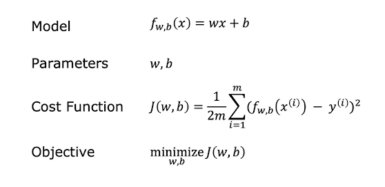
When we have only one input variable we call this model/algorithm univariate linear regression. In a univariate linear regression model, we have $f(x) = wx + b$, where $x$ is the input variable, and $w, b$ are numbers which are called parameters of the model. So $f(x)$ is a linear function of $x$. It's also written sometimes as $f_{w,\ b}(x) = wx + b$. By varying the parameters $w$ and $b$ we get different linear models. The parameter $w$ is called the slope, and $b$ is called the y-intercept because $b=f(0)$ and so $b$ is the point where the graph of $f(x)$ intercepts the $y$ axis.

When we have more than one input variable (more than one feature) the model is called multivariate linear regression. In this case we try to predict the values of the target variable $y$ based on several input variables $x_1, x_2, \dots, x_k$. Here we have $k \in \mathbb{N}, k \ge 2$.

In a univariate linear regression model the most commonly used cost function is the mean squared error cost function.

$$J(w,b) = \frac{1}{m} \cdot \sum_{i=1}^m (\widehat{y}^{(i)} - y^{(i)})^2$$

In the last formula

$\widehat{y}^{(i)} = f_{w,b}(x^{(i)}) = wx^{(i)} + b$ 

for $i=1,2,\dots,m$.

So for the cost function we also get the following expression 

$$J(w,b) = \frac{1}{m} \cdot \sum_{i=1}^m (f_{w,b}(x^{(i)}) - y^{(i)})^2$$

Note that $J(w,b) \ge 0$

In practice an additional division by 2 is performed in the formulas given above. This is done just for practical reasons, to make further computations simpler. In this way we get the final version of our cost function.

$$J(w,b) = \frac{1}{2m} \cdot \sum_{i=1}^m (\widehat{y}^{(i)} - y^{(i)})^2$$

$$J(w,b) = \frac{1}{2m} \cdot \sum_{i=1}^m (f_{w,b}(x^{(i)}) - y^{(i)})^2$$

Then the task is to find values of $w,b$ such that the value of $J(w,b)$ is as small as possible. 

The smaller the value of $J(w,b)$, the better the model.

All this info about univariate linear regression can be summarized with the following picture 

(pictures credits go to Andrew Ng's Coursera ML Course).

An application of the AM-GM inequality

I found this problem and its solution in a FB group dedicated to maths. Here they are. 

Problem: 

If $a,b,c \gt 0$ prove that 

$$\frac{a^2 + b^2}{c} + \frac{b^2 + c^2}{a} + \frac{c^2 + a^2}{b} \ge 2(a+b+c)$$

Solution:

By the AM-GM inequality we have that

$$\frac{a^2}{c} + c + \frac{b^2}{c} + c \ge 2\sqrt{a^2} + 2\sqrt{b^2} = 2(a+b)$$

$$\frac{b^2}{a} + a + \frac{c^2}{a} + a \ge 2\sqrt{b^2} + 2\sqrt{c^2} = 2(b+c)$$

$$\frac{c^2}{b} + b + \frac{a^2}{b} + b \ge 2\sqrt{c^2} + 2\sqrt{a^2} = 2(c+a)$$

When we sum up these 3 inequalities we get the desired inequality.

Note: This solution is due to Ghimisi Dumitrel, Professor at Colegiul National Ionita Asan, Caracal.

Machine Learning Notes 1

1) Machine learning (ML) related definitions

Definition A (Athur Samuel, 1959): Machine learning is the field of study which gives computers the ability to learn without being explicitly programmed.

Definition B (Tom Mitchell, 1998): Well-posed machine learning problem: A computer program is said to learn from experience E with respect to some task T and some performance measure P, if its performance on T, as measured by P, improves with experience E.

2) Types of ML algorithms

In general any ML algorithm can be classified into one of the following two categories

• Supervised learning (the "right answers" are given in the initial data set; i.e. the data set is labeled)
• Regression: trying to predict the values of some quantity which we view as a continuous function
• Classification: trying to predict the values of some quantity whose possible values form a small finite discrete set (that set could be e.g. {Yes, No}; {0,1,2,3}; {Cat, Dog, Other}; etc.); trying to classify a set of data points into a small finite number of classes
• Unsupervised learning (the "right answers" are not given in the initial data set; i.e. the data set is unlabeled); in unsupervised learning the task is to automatically find some structure in the unlabeled data set that is given
• Clustering: a data set is given, the task is to break it down into several separate clusters (i.e. into several separate disjoint data sets). Examples: 1) Google news (news articles from various sources are grouped together if they are about the same story); 2) Market segmentation: find market segments/clusters in a dataset which contains data about all customers of a given company.
• Non-clustering: 
• Independent component analysis (used in signal processing). Example: separating different voices (or say different audio tracks) out of one (or a few) given chaotic audio recordings (see e.g. (1) cocktail party effect, (2) cocktail party problem and algorithm). The so-called "cocktail party algorithm" allows you to find structure in a chaotic environment (identifying individual voices and music from a mesh of sounds at a cocktail party).
• Anomaly detection (detect unusual data points in a given dataset). Anomaly detection (also referred to as outlier detection and sometimes as novelty detection) is generally understood to be the identification of rare items, events or observations which deviate significantly from the majority of the data and do not conform to a well defined notion of normal behavior (Source: Wikipedia). 
• Dimensionality reduction (compress data points using fewer numbers). Dimensionality reduction, or dimension reduction, is the transformation of data from a higher-dimensional space into a lower-dimensional space so that the lower-dimensional representation retains some meaningful properties of the original data, ideally close to its intrinsic dimension (Source: Wikipedia).

3) GNU Octave

This is a powerful framework for quick prototyping of solutions/algorithms for ML problems (see here: GNU Octave)

NumPy operators and their corresponding NumPy universal functions (ufuncs)

NumPy operators and their corresponding NumPy universal functions (ufuncs)

This table was compiled from the 3 tables shown on pages 53, 72, 75 of the book Python Data Science Handbook by Jake VanderPlas. I put it here just for my own reference.

Arithmetic Operator	Equivalent ufunc	Description
+	np.add	Addition (e.g., 1 + 1 = 2)
-	np.subtract	Subtraction (e.g., 3 - 2 = 1)
-	np.negative	Unary negation (e.g., -2)
*	np.multiply	Multiplication (e.g., 2 * 3 = 6)
/	np.divide	Division (e.g., 3 / 2 = 1.5)
//	np.floor_divide	Floor division (e.g., 3 // 2 = 1)
**	np.power	Exponentiation (e.g., 2 ** 3 = 8)
%	np.mod	Modulus/remainder (e.g., 9 % 4 = 1)
Comparison Operator	Equivalent ufunc
==	np.equal
!=	np.not_equal
<	np.less
<=	np.less_equal
>	np.greater
>=	np.greater_equal
Logical Operator	Equivalent ufunc	See also
&	np.bitwise_and	np.logical_and
|	np.bitwise_or	np.logical_or
^	np.bitwise_xor	np.logical_xor
~	np.bitwise_not	np.logical_not

NumPy rules of broadcasting

These rules are listed in the book Python Data Science Handbook by Jake VanderPlas (see page 65).

Broadcasting in NumPy is simply a set of rules for applying binary universal functions (like addition, subtraction, multiplication, etc.) on NumPy arrays of different sizes.

Here are the NumPy broadcasting rules. 

• Rule 1: If the two arrays differ in their number of dimensions, the shape of the
one with fewer dimensions is padded with ones on its leading (left) side.

• Rule 2: If the shape of the two arrays does not match in any dimension, the array
with shape equal to 1 in that dimension is stretched to match the other shape.

• Rule 3: If in any dimension the sizes disagree and neither is equal to 1, an error is
raised.