Supervised learning terminology/notation
- Training set is the dataset used to train the model
- $x$ - the input variable, the input feature
- $y$ - the output variable, the target variable
- $m$ - the total number of the training examples (training data points)
- $(x^{(i)}, y^{(i)})$ - the $i$-th training example (for $i=1,2,\dots, m$); here the expression $(i)$ is just a superscript, it does not denote exponentiation
- $f$ - hypothesis function, prediction function; also $f$ is called the model
- $\widehat{y} = f(x)$, where $x$ is the input variable and $\widehat{y}$ is the prediction for the target variable $y$
- $\widehat{y}^{(i)} = f(x^{(i)})$, where $x^{(i)}$ is the $i$-th training example, and $\widehat{y}^{(i)}$ is the prediction value corresponding to $x^{(i)}$
- Cost function is a function which estimates how well a given model predicts the values for the target variable $y$; this is a function which measures how well the model fits the training data. Cost function is a general concept which is applicable to any supervised learning model.
Linear regression with one variable (univariate linear regression)
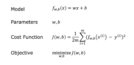
When we have only one input variable we call this model/algorithm univariate linear regression. In a univariate linear regression model, we have $f(x) = wx + b$, where $x$ is the input variable, and $w, b$ are numbers which are called parameters of the model. So $f(x)$ is a linear function of $x$. It's also written sometimes as $f_{w,\ b}(x) = wx + b$. By varying the parameters $w$ and $b$ we get different linear models. The parameter $w$ is called the slope, and $b$ is called the y-intercept because $b=f(0)$ and so $b$ is the point where the graph of $f(x)$ intercepts the $y$ axis.
When we have more than one input variable (more than one feature) the model is called multivariate linear regression. In this case we try to predict the values of the target variable $y$ based on several input variables $x_1, x_2, \dots, x_k$. Here we have $k \in \mathbb{N}, k \ge 2$.
In a univariate linear regression model the most commonly used cost function is the mean squared error cost function.
$$J(w,b) = \frac{1}{m} \cdot \sum_{i=1}^m (\widehat{y}^{(i)} - y^{(i)})^2$$
In the last formula
$\widehat{y}^{(i)} = f_{w,b}(x^{(i)}) = wx^{(i)} + b$
for $i=1,2,\dots,m$.
So for the cost function we also get the following expression
$$J(w,b) = \frac{1}{m} \cdot \sum_{i=1}^m (f_{w,b}(x^{(i)}) - y^{(i)})^2$$
Note that $J(w,b) \ge 0$
In practice an additional division by 2 is performed in the formulas given above. This is done just for practical reasons, to make further computations simpler. In this way we get the final version of our cost function.
$$J(w,b) = \frac{1}{2m} \cdot \sum_{i=1}^m (\widehat{y}^{(i)} - y^{(i)})^2$$
$$J(w,b) = \frac{1}{2m} \cdot \sum_{i=1}^m (f_{w,b}(x^{(i)}) - y^{(i)})^2$$
Then the task is to find values of $w,b$ such that the value of $J(w,b)$ is as small as possible.
The smaller the value of $J(w,b)$, the better the model.
All this info about univariate linear regression can be summarized with the following picture
(pictures credits go to Andrew Ng's Coursera ML Course).

